Three lines of generative models, and the one that samples Boltzmann生成式算法的三条线，以及用来做玻尔兹曼采样的那一条

Status: a working map written around four eprints. I will revise it when a claim here is overtaken by a paper I have actually read.

The argument of this note is linear. Generative models developed along a few distinct lines. The middle one is Boltzmann sampling: the density is known only up to $Z$. That line has three difficulties; on the lattice they have specific faces. The samplers we built — VAN, SPS, NHMC — are attempts to move those faces. Among the remaining costs, the expensive one is no longer only the Markov chain. It is the architecture: gauge-equivariant training is slow, so the next design step is to ask which operator bases a trained network actually uses, and to put those bases in by hand.

Three lines, by what is given

I sort generative models by the object one is handed, not by the brand name of the network.

Line 1 — samples, no density. Images, text, recorded molecular snapshots. The job is to fit $p_{\mathrm{data}}$. Autoregressive models, VAEs, GANs, diffusion, and flow matching all live here. Quality is likelihood of data, or a perceptual proxy. There is no Boltzmann weight to be faithful to.

Line 2 — an unnormalized density, often no samples. This is the middle line, and the one used for physics. The target is

\[\pi(x)=\frac{1}{Z}\,e^{-E(x)},\qquad Z=\int dx\,e^{-E(x)},\]

with $E$ (or a lattice action $S$) known and $Z$ intractable. Boltzmann generators, reverse-KL normalizing flows, variational autoregressive networks, and path-space samplers belong here. Quality is not that the fields look right. It is that a named correction still represents $\pi$ after you close the notebook.

Line 3 — a symmetry or a process law. Gauge covariance, $Z_2$, permutation symmetry, or a prescribed SDE. The model is no longer free to use any function of the input. Equivariant flows, loop-force networks, and score models with a built-in process sit here. This line is not an alternative to Boltzmann sampling; it is the constraint that appears when line 2 is imposed on a field with symmetry. It is also where the architecture becomes expensive.

A paper can sit on more than one line. Diffusion trained on HMC configurations is line 1 pointed at a lattice. The same SDE trained only from $S[\phi]$ is line 2. A gauge-equivariant version of either is line 3 wrapped around them. The map is for placing the paper, not for ranking brands.

The middle line: Boltzmann sampling

On line 2 the generative object is a proposal $q_\theta$, cheap to sample, together with enough density or path-probability information to correct it. That is the opposite of image generation. The unnormalized density is given; the job is to move probability mass without destroying correctness.

Training usually minimizes a reverse KL, which is available because $S$ is known:

\[D_{\mathrm{KL}}(q_\theta\parallel\pi)=\mathbb{E}_{q_\theta}\bigl[\log q_\theta-\log\pi\bigr].\]

Reverse KL is mode-seeking. A model that covers one phase, or one topological sector, can look excellent on the loss and still be unusable as an ensemble. So every construction I trust ends with a statistical correction: independent Metropolis–Hastings, self-normalized importance sampling, a Metropolis-adjusted local kernel on top of the neural proposal, or a path-space work weight. If the weights collapse or the acceptance vanishes, the proposal has failed. I treat that failure as evidence about $q_\theta$, not as a reason to drop the correction.

Three difficulties, and their lattice faces

Boltzmann sampling is hard for three reasons that are older than neural nets. On the lattice they have specific faces.

Critical slowing down. Local, equilibrium Markov chains mix on the scale of the correlation length. Toward a second-order point — or, for an asymptotically free gauge theory, toward the continuum $\xi/a\to\infty$ — the integrated autocorrelation time grows as a power of $\xi/a$. You pay more and more trajectories for one independent configuration. In two-dimensional $\phi^4$, the finite-volume face of this is the pseudocritical strip: susceptibility peaks, the magnetization distribution becomes hard, and HMC’s $\tau_{\mathrm{int}}$ rises.

Topological freezing. In gauge theories the same slowing down often appears as a stuck topological charge $Q$. The chain is then not ergodic. Observables that couple to topology are biased in a way that is easy to miss if one only looks at local correlators. Scalar $\phi^4$ has a cheaper analogue: $Z_2$ sector collapse, where a reverse-KL model sits in one broken-phase well and never sees the other.

The sign problem. If $S$ is complex, $e^{-S}$ is not a probability. Finite-density QCD, real-time evolution, and a $\theta$-term are this door. Almost none of the generative constructions below, as they are usually trained, address it. Treating a complex weight as if it were a Boltzmann factor is a different problem. I keep it on the list so the map does not pretend the three difficulties are equally open.

A method is interesting only if it changes one of those three costs, or gives a controlled estimator of $Z$ itself.

What we changed on that line

The three samplers below are all line-2 objects: data-free proposals for an unnormalized Boltzmann density, plus a named correction. They differ by what is learned.

VAN — factorize, then correct locally. With Shiyang Chen, arXiv:2512.19575 extends variational autoregressive networks from discrete spins to continuous $\phi^4$. The joint is written as a chain of conditionals, $q_\theta(\phi)=\prod_i q_\theta(\phi_i\mid\phi_{<i})$, and trained from the action alone by a REINFORCE-style variational free energy. That is the local face of line 2: generation looks like a single-site sweep, which is why we expected it to avoid some of the mode-covering failures of a single global map.

The learned $q_\theta$ is not $\pi$. Single-site and block Metropolis–Hastings updates on top of the VAN proposal remove the residual bias we saw in pure VAN sampling, while the effective sample size stays high in the range we studied. Transfer learning is the other practical move: the KL between the magnetization distribution and a Gaussian reference tracks how hard a $(\kappa,L)$ point is, and fine-tuning a model pretrained at one $\kappa$ is cheaper than training from a Gaussian field. On Ising and on $\phi^4$ up to $L=10$, $\kappa\in[0.20,0.30]$, the corrected ensembles agree with standard Monte Carlo within errors, and we do not see clear critical slowing down in that window. That is not a continuum-limit claim.

SPS — learn the path, then correct on path space. With Chen, Aarts, Lucini, and Zhou, arXiv:2606.13790 changes the learned object. Instead of an endpoint density, SPS learns forward and backward stochastic dynamics between a Gaussian prior and the Boltzmann target, and trains by lowering the path-space irreversibility — the KL between the two trajectory measures, equivalently an entropy-production bound. No HMC configurations are used. After training, an extended-space independence Metropolis–Hastings step restores exactness, provided the proposal covers the support.

On two-dimensional $\phi^4$ with the $L\times 8$ finite-temperature geometry, SPS matches HMC on magnetization, susceptibility, and the free-energy estimator through the pseudocritical region, up to $L=64$, with a much shorter autocorrelation than HMC. Uncorrected SPS already sits close to HMC on those observables; IMH is there because closeness is not exactness. This is a 2d scalar result. It is a stochastic-quantization-inspired route to a data-free proposal, not a 4d gauge sampler.

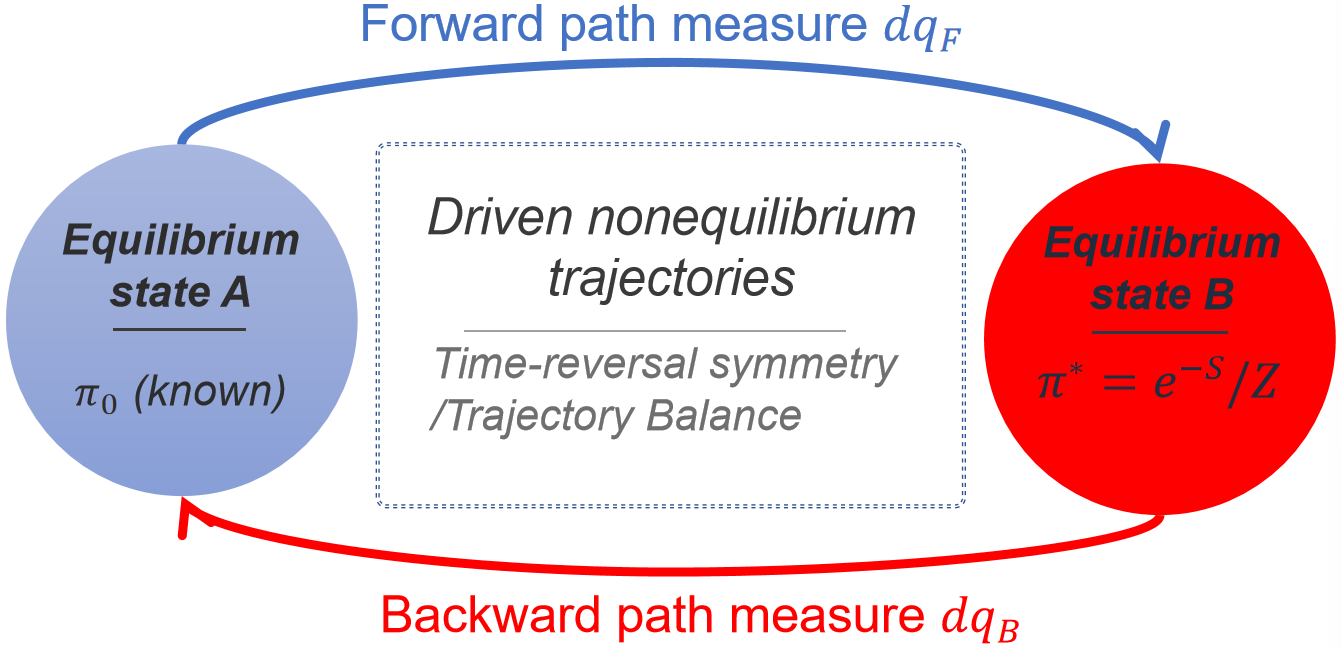
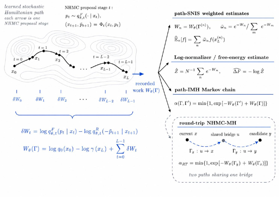
NHMC — keep the path correction, change the process to a Hamiltonian path. arXiv:2607.15682 is the Hamiltonian version of the same train-then-correct idea. The proposal is a stochastic Hamiltonian-style path: draw a learned conditional momentum, apply a reversible volume-preserving kick–drift map, record the forward and reverse path probabilities. The log ratio is a dimensionless generalized work $W_\theta$. During training, its mean is a path-space KL. After training, the same $W_\theta$ is the weight for path-SNIS, the acceptance for path-IMH, and the correction inside a proved shared-bridge round-trip Metropolis kernel that acts on configurations and leaves $\pi$ invariant.

On double-well and finite-volume $\phi^4$ targets the corrected estimates are good when path overlap is sufficient. When overlap is poor, weight degeneracy, low acceptance, and long autocorrelation are the result: they expose proposal failure instead of hiding it. The molecular internal-coordinate study and the compact $U(1)$ round-trip sit in the paper as feasibility boundaries, not as completed applications.

Taken together, the three papers move different faces of the same difficulty. VAN attacks mixing by a local, factorized proposal plus a cheap MH polish, and attacks parameter scans by transfer. SPS and NHMC attack global transport: they learn a process whose path probability is recorded, so the correction does not need an endpoint Jacobian. None of them claims to have opened the sign-problem door. None of them is 4d $SU(3)$ at fine $a$.

The architecture problem, and why I started reading bases

Among those improvements a different cost showed up. To put line 3 into line 2 — to respect gauge covariance, or even $Z_2$, at the level of the function space — the standard move is an equivariant network. That is the right kinematic constraint. It is also slow. Gauge-equivariant coupling layers and loop-valued convolutions are large, their Jacobians or score maps are expensive, and a full equivariant retrain is a poor way to search for a better inductive bias. I wanted a cheaper question: after a network has been trained, which operator bases does the trained field actually use?

That is operator spectroscopy, arXiv:2605.11199. The object of study is no longer the ensemble. It is the trained field-space function itself — a flow-matching velocity, a diffusion score, or a normalizing-flow action residual $\Delta S_q=-\log q_\theta-S-C$. Project it onto a dictionary fixed before the fit, chosen from symmetry, exact Gaussian path limits, finite-volume modes, and gauge covariance:

\[\mathcal{T}_\theta(\tau,\phi)=\sum_n c_n(\tau)\,\mathcal{O}_n[\phi]+r_\theta(\tau,\phi).\]

A sector is kept only if it lowers the held-out residual, moves the observable it is supposed to move, and is not reproduced by wrong-parity, shuffled, or random controls.

The $\phi^4$ result is the one that changed how I think about architecture. A trained straight-flow teacher is not described by a local force basis alone. After the local transport piece, the residual splits into two infrared channels: a deflated zero-mode polynomial $P_5(M;t)$ that carries the Binder tail, and the lowest nonzero Fourier shell $\phi^\perp_{\lvert n\rvert^2=1}$ that carries the finite-$k$ correlator. They are essentially orthogonal at $L=8$. Wrong-parity zero modes and random Fourier directions do not fake the same reductions. So a network that only spends capacity on a local stencil is paying for the wrong function space, and a fully equivariant giant net may be paying for a much larger space than the trained dynamics ever uses.

The same projection reads other failures. A collapsed reverse-KL flow shows a forbidden odd zero-mode term in $\Delta S_q$ — the operator signature of a spurious magnetic field — with the odd-block $R^2$ dropping from $0.865$ to below $10^{-3}$ once $Z_2$ is imposed. A variance-exploding diffusion teacher follows the force-resolvent ordering predicted by the free theory, which is a different leading basis from flow matching; the distinction is path-selected, not architectural. For gauge-equivariant teachers the scalar dictionary is replaced by Lie-algebra-valued loop forces. Wilson-loop-force operators lower the tangent-field residual; raw links, shuffled loops, and random controls do not. Equivariance fixes the kinematic space. The projection says which covariant directions the trained dynamics actually occupy.

That is the design loop I want next. Do not start from a larger equivariant U-Net. Start from the retained sectors — local transport, a short zero-mode tower, the lowest soft shell, a small set of loop forces — and build a network whose layers are those bases, with a handful of learned coefficients along the probability path. Training should be faster because the function space is the one the teacher already chose. Sampling should be better because the infrared pieces that local force misses, and that full equivariance buries inside hundreds of thousands of weights, sit in the architecture on purpose.

The spectroscopy paper is the diagnostic, not the new sampler. VAN, SPS, and NHMC are the line-2 machines. The next architecture is the attempt to stop paying the line-3 tax in full.

What I am not claiming

Two-dimensional $\phi^4$ and a compact $U(1)$ pilot are not 4d $SU(3)$. A shorter autocorrelation on an $L\times 8$ strip is not the continuum limit. An operator basis that is stable across a $\kappa$ sweep is not yet a trained sampler with that basis hard-wired. The sign problem is still a different door.

If a later architecture built from these sectors trains faster and samples better, that will be a separate note, with the same correction law as above.